This study demonstrates how a researcher could use miXGENE to work on a particular set of experiments. Section 1 describes the domain under study and properties of the given datasets. The experimental procedure that remains the same for all experiments is presented in Section 2. Section 3 contains individual experiments description and collected results. The entire case study along with the achieved results is discussed in Section 4.

Gene expression analysis often operates with different measurement units. In this study the mRNA, miRNA and DNA methylation are considered. There exist different approaches how to integrate such data, some of them can utilize background knowledge. In the following experiments a few approaches that differ in the way of preprocessing and classification are compared.

The corresponding miXGENE experiments are the following:

Role of quantile normalisation. Link
Simple merge. Link
The role of feature selection. Link
Integration of mRNA and miRNA data using prior knowledge in the form of binary relation. Link

1 Dataset description

The source data for this study was provided by Dr. Jakub Tolar, University of Minnesota. It deals with germ cell tumors (GCT). The provided data contain samples with the following GCT types: yolk sac tumor (YST), bening and malignant teratoma, dysgerminoma, mixed tumors, and control samples without tumors.

Germ cells are specialized in production of cell used for human reproduction (Cinalli et al., 2008). Germ cells are formed at the fringe of embryo and then transported into growing gonads (ovary or testis). When a germ cell reaches gonad it acquires sex specialization. But sometimes some germ cells do not arrive to gonads and remain in wrong tissue. So GCT mainly declare itself in gonads, but can also present in other locations.

GCT causes diverse diagnostic challenges for pathologist, as well as introduce number of academic question for research about connection between GCT and gonads development (Ulbright, 2005).

The measurements were done on 40 samples and consist of three expression profiling datasets:

mRNA: 85 features,
miRNA: 734 features,
DNA methylation: 1408 features.

The samples are categorised by:

age: $\{0,1, ...\}$ ,
sex: $\{male, female\}$ ,
location: $\{ovar, testis, other, normal\}$ ,
histology: $\{normal, mixed, YST, benign teratoma, teratoma, dysgerminoma\}$ .

2 Experimental protocol

2.1 Target class assignments

To compare integration methods we need to define a set of binary target classes first. Since it is not obvious how to do such an assignment from the given phenotype information, we created a few possible target class assignments or tasks:

Table 1: Prepared tasks for class predication based on phenotype

Task	Common	Class 1		Class 2
	properties	histology	samples #	histology	samples #
T1		benign teratoma	9	normal	4
T2		teratoma	10	normal	4
T3		mixed	3	normal	4
T4		dysgerminoma	7	normal	4
T5		benign teratoma or teratoma	19	YST	7
T6	location = ovary	benign teratoma or teratoma	8	dysgerminoma	7
T7	sex = male	benign teratoma or teratoma	5	YST	4

2.2 Classification

In this study two classification algorithms were used: Linear SVM and Random forest.

SVM: Support vector machine, finds a linear decision surface (hyperplane) in a high dimensional feature space which has largest distance to the nearest training point of any class. This algorithm was proposed by Cortes and Vapnik (Cortes and Vapnik, 1995). Currently SVM is widely used in gene expression analysis, due to its ability to discriminate datasets when the number of samples is much less than the number of dimensions.
RF: Random forest in an example of ensemble method, it combines a number of randomized decision trees. This algorithm was originally proposed by Breiman (2001). RF is not often used in genomics, but there are some studies where RF was applied (Hsueh et al., 2013). RF has some promising properties: it does not overfit, does implicit feature selection, and allows extensive missing values and unbalanced data.

During all the experiments, each compared configuration was tested with 5-times repeated 5-fold cross-validation. This was done by the Cross Validation block and classifiers immersed into its sub-scope.

2.3 Comparison of results

To compare results across all experiments Matthews correlation coefficient (MCC) was used as a performance metric suitable for unbalanced classes. It computes prediction quality of the classification results with two classes. The MCC was chosen for similar reasons as in Kléma et al. (2014):

sizes of the target classes differ,
experiments deals with dependent tasks and settings.

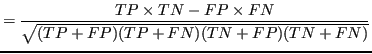
MCC $\displaystyle = \frac{ TP \times TN - FP \times FN } {\sqrt{ (TP + FP) ( TP + FN ) ( TN + FP ) ( TN + FN ) } }$

Where :

TP: the number of true positives,
TN: the number of true negatives,
FP: the number of false positives,
FN: the number of false negatives.

MCC metric returns a float number from interval ; means the perfect prediction, 0 suggests random prediction, and stands for the inverse prediction. In the binary classification tasks under consideration there are and classes, but due to symmetry it does not affect MCC metric.

Results of the each experiments are presented in two parts:

Performance table with the achieved MCC score for the combination of different Tasks (Section 2.1), Classifiers (Section 2.2) and individual configurations of each experiment.
Pairwise comparison between the compared configuration of the particular experiment. It is directly computed from the performance table.

3 Experiment workflows and results

3.1 Role of quantile normalisation

Normalization has been done outside of miXGENE only for mRNA and miRNA, so we have a pair of datasets. To compare them we use Custom iterator block with two cells: the first one is bound to raw datasets while the second one is bound to the normalized ones.

**Figure 1:** Workflow of *Role of quantile normalisation* experiment.

The workflow structure is presented in Figure 1, the obtained results are presented in Table 2, and the miXGENE experiment is here. From the 42 designed configurations, the usage of normalized data is preferable 26 times, raw data reach better score 7 times and tie appears 9 times.

**Table 2:** Role of the data normalisation experiment. Performance table, w.r.t. MCC score
$\begin{table}\hspace*{-0.35in} \centering \pgfplotstabletypeset[ col sep=comma,... ...fixed,zerofill=true,precision=3, ]{data/exp4_MCC_compact.csv} \par\end{table}$

**Table 3:** Role of the data normalisation experiment. Pairwise comparison of the normalized and raw data, w.r.t. MCC score
$\begin{table}\centering \pgfplotstabletypeset[ col sep=comma, ignore chars={[,... ...wcolor[gray]{0.9} }}, fixed,precision=3, ]{data/exp4_pw.csv} \par\end{table}$

3.2 Simple merge

During this experiment, the accuracy reached with the independent use of the individual datasets and various ways of their simple merge was compared. The merge is simply done by dataset concatenation since each dataset has the identical set of samples.

This method was presented in Lanza et al. (2007) and operates with mRNA and miRNA datasets. In this experiment, there are 4 merged datasets: one containing all three sources (mRNA, miRNA, DNA methylation) and 3 dataset obtained from source pairs: mRNA and miRNA, mRNA and DNA methylation, miRNA and DNA methylation.

**Figure 2:** Workflow schema of *Simple merge* experiment.

The workflow structure is presented in Figure 2, the obtained results are shown in Table 4 and 5, and the miXGENE experiment is here. In the result tables, the name refers to the dataset obtained by the concatenation of all the three source datasets.

**Table 4:** Simple merge experiment. Performance table, w.r.t. MCC score
$\begin{table}\centering \pgfplotstabletypeset[ col sep=comma, ignore chars={[,... ...fixed,zerofill=true,precision=3, ]{data/exp1_simple_merge_MCC.csv}\end{table}$

**Table 5:** Simple merge experiment. Pairwise comparison, w.r.t. MCC score
$\begin{table}\centering \pgfplotstabletypeset[ col sep=comma, ignore chars={[,... ...wcolor[gray]{0.9} }}, fixed,precision=3, ]{data/exp1_pw.csv} \par\end{table}$

3.3 The role of feature selection

In the second experiment, we start with individual mRNA, miRNA and methyl datasets and one dataset that merge all of them as described in the previous section. Two-source merged datasets were omitted.

To overcome problems of the high-dimensional feature space we use feature selection (FS). FS is an approach to reduce dimensionality of data by discarding of irrelevant features and applicable in the domain of gene expression analysis (Guyon and Elisseeff, 2003).

In miXGENE FS is implemented by the two kinds of blocks:

Compute statistic about features, so we obtain generic TableResult where each rows represents features and columns contains computed statistics values. During the study we used the following blocks:
- Restricted Svmrfe ranking: it repeatedly runs SVM, at each run ranks features and discards features with the lowest weight. The number of runs is restricted by the user to limit execution time.
- T-test ranking: it computes T-test statistic for each feature under the assumption of feature independence. Then it reorders the features according to the obtained statistic values.
- Random rank: creates a random ranking. We use this block as a benchmark.
All of them produce one output: the , which provides a simple feature ordering.
Prune dataset by the given rank. It is done through the block Feature selection by ranking cut which prunes dataset by the given TableResult, statistic name and threshold value.

**Figure 3:** Workflow schema of *Role of feature selection* experiment.

The workflow structure is presented in Figure 3, the obtained results are presented in Table 6 and 7, and the miXGENE experiment is here.

**Table 6:** The Role of feature selection. Performance table, w.r.t. MCC score
$\begin{table}\centering \pgfplotstabletypeset[ col sep=comma, ignore chars={[,... ... }}, fixed,zerofill=true,precision=3, ]{data/exp2_MCC_p.csv} \par\end{table}$

**Table 7:** The role of feature selection. Pairwise comparison of the ranking methods, w.r.t. MCC score
$\begin{table}\centering \pgfplotstabletypeset[ col sep=comma, ignore chars={[,... ...wcolor[gray]{0.9} }}, fixed,precision=3, ]{data/exp2_pw.csv} \par\end{table}$

3.4 Integration of mRNA and miRNA data using PK in the form of binary relation

This experiment is based on the work (Kléma et al., 2014). The simple merge of mRNA and miRNA does not always produce better data for machine learning because the feature space grows without adding more samples and uninformed concatenation. To reduce the problem space by utilization of prior knowledge (PK) two aggregation methods were proposed: "Subtractive aggregation" and "SVD aggregation". Both of them utilize knowledge about which miRNA targets which mRNA.

As a source of interaction data we use publicly available databases (TarBase (Vergoulis et al., 2012) and miRWalk (Dweep et al., 2011) ). TarBase contains only validated interaction, it is more reliable but has much fewer records than miRWalk which also collects predicted interactions.

DNA methylation datasets were omitted in this experiment, since aggregation methods do not expect such an input yet. During this experiment dataset contains only mRNA and miRNA data.

mRNA and miRNA datasets were pruned by the miRNA-to-mRNA targets information, so each of them keeps genes that are presented in the interaction matrix only.

Since FS with ttest ranking has shown better results in the previous experiment we apply it again to the individual data types and aggregated datasets.

**Figure 4:** Workflow schema of *Integration of mRNA and miRNA data using PK in form of binary relation* experiment.

The workflow structure is presented in Figure 4, the obtained results are split according to the interaction databases and depicted in Tables 8, 9, 11, 12, and the miXGENE experiment is here. The interaction databases are compared in Table 10, which concludes only configurations with aggregation methods that utilize prior knowledge.

**Table 8:** Integration of mRNA and miRNA data using PK: TarBase interaction. Performance table, w.r.t. MCC score
$\begin{table}\centering \pgfplotstabletypeset[ col sep=comma, ignore chars={[,... ...fixed,zerofill=true,precision=3, ]{data/exp3_MCC_TarBase.csv} \par\end{table}$

**Table 9:** Integration of mRNA and miRNA data using PK: miRWalk interaction. Performance table, w.r.t. MCC score
$\begin{table}\centering \pgfplotstabletypeset[ col sep=comma, ignore chars={[,... ...fixed,zerofill=true,precision=3, ]{data/exp3_MCC_MirWalk.csv} \par\end{table}$

**Table 10:** Integration of mRNA and miRNA data using PK. Pairwise comparison of the target matrices, w.r.t. MCC score. Limited only to the configurations with aggregation methods that utilize PK (sub, svd).
$\begin{table}\centering \pgfplotstabletypeset[ col sep=comma, ignore chars={[,... ...lor[gray]{0.9} }}, fixed,precision=3, ]{data/exp3_pw_DB.csv} \par\end{table}$

**Table 11:** Integration of mRNA and miRNA data using PK experiment. TarBase interaction database. Pairwise comparison, w.r.t. MCC score
$\begin{table}\hspace*{-0.5in} \centering \pgfplotstabletypeset[ col sep=comma,... ...r[gray]{0.9} }}, fixed,precision=3, ]{data/exp3_TAR_pw.csv} \par\end{table}$

**Table 12:** Integration of mRNA and miRNA data using PK experiment. MirWalk interaction database. Pairwise comparison, w.r.t. MCC score
$\begin{table}\centering \pgfplotstabletypeset[ col sep=comma, ignore chars={[... ...or[gray]{0.9} }}, fixed,precision=3, ]{data/exp3_MIR_pw.csv} \par\end{table}$

4 Conclusion

In the germ cell tumor case study, the following conclusions were achieved based on comparison of the individual classification target vectors:

Quantile normalisation of expression profiles improves predictive accuracy in the most cases. It is reasonable to employ the normalisation block.
Simple integration of heterogeneous datasets by concatenation is of no use without further enhancements (feature selection, application of prior knowledge, etc.).
Surprisingly, feature selection by the simple t-test ranking outperforms the more sophisticated SVM-RFE method. According to expectations, both the informed methods of feature selection outperform random feature ranking.
Aggregation methods with PK perform better than simple merge by concatenation.
Within the case study it is hard to conclusively select the mRNA-miRNA target interaction database to be used for the aggregation. SVM classifier gives the perfect predictions with both the interaction databases. With the Random Forest classifier MirWalk database wins more times.
Linear SVM classifier outperforms Random Forest in all the experiments in the most configurations. Pairwise comparison is depicted in Table 13.
The overall absolute accuracy is highly promising. In the fourth experiment almost any configuration with SVM classifier showed MCC 1 which corresponds to the perfect split between the target classes.

**Table 13:** Pairwise comparison of the classification algorithms across all experiments, w.r.t. MCC score
$\begin{table}\centering \pgfplotstabletypeset[ col sep=comma, ignore chars={[,... ...gray]{0.9} }}, fixed,precision=3, ]{data/pw_classifiers.csv} \par\end{table}$

Bibliography

Leo Breiman.: Random forests.
Machine Learning, 45 (1): 5-32, 2001.
ISSN 0885-6125.
doi: rm10.1023/A:1010933404324.
URL http://dx.doi.org/10.1023/A
Ryan M Cinalli, Prashanth Rangan, and Ruth Lehmann.: Germ cells are forever.
Cell, 132 (4): 559-62, March 2008.
ISSN 1097-4172.
doi: rm10.1016/j.cell.2008.02.003.
URL http://www.ncbi.nlm.nih.gov/pubmed/18295574.
Corinna Cortes and Vladimir Vapnik.: Support-vector networks.
Machine learning, 297: 273-297, 1995.
URL http://link.springer.com/article/10.1007/BF00994018.
Harsh Dweep, Carsten Sticht, Priyanka Pandey, and Norbert Gretz.: miRWalk Database: Prediction of possible miRNA binding sites by "walking" the genes of three genomes.
Journal of Biomedical Informatics, 44 (5): 839 - 847, 2011.
ISSN 1532-0464.
doi: rmhttp://dx.doi.org/10.1016/j.jbi.2011.05.002.
URL http://www.sciencedirect.com/science/article/pii/S1532046411000785.
Isabelle Guyon and André Elisseeff.: An introduction to variable and feature selection.
J. Mach. Learn. Res., 3: 1157-1182, March 2003.
ISSN 1532-4435.
URL http://dl.acm.org/citation.cfm?id=944919.944968.
Huey-Miin Hsueh, Da-Wei Zhou, and Chen-An Tsai.: Random forests-based differential analysis of gene sets for gene expression data.
Gene, 518 (1): "179 - 186", 2013.
ISSN 0378-1119.
URL "http://www.sciencedirect.com/science/article/pii/S0378111912014552".
Proceedings of the 23rd International Conference on Genome Informatics (GIW 2012).
Jiri Klema, Jan Zahalka, Michael Andel, and Zdenek Krejcík.: Knowledge-Based Subtractive Integration of mRNA and miRNA Expression Profiles to Differentiate Myelodysplastic Syndrome.
In Proceedings of the International Conference on Bioinformatics Models, Methods and Algorithms, pages 31-39. Porto: SciTePress - Science and Technology Publications, 2014.
URL http://ida.felk.cvut.cz/klema/publications/Biotex/Bioinformatics2014_final.pdf.
Giovanni Lanza, Manuela Ferracin, Roberta Gafa;, Angelo Veronese, Riccardo Spizzo, Flavia Pichiorri, Chang-gong Liu, George A Calin, Carlo M Croce, and Massimo Negrini.: mRNA/microRNA gene expression profile in microsatellite unstable colorectal cancer.
Molecular cancer, 6: 54, January 2007.
ISSN 1476-4598.
doi: rm10.1186/1476-4598-6-54.
URL http://www.pubmedcentral.nih.gov/articlerender.fcgi?artid=2048978&tool=pmcentrez&rendertype=abstract.
Thomas M Ulbright.: Germ cell tumors of the gonads: a selective review emphasizing problems in differential diagnosis, newly appreciated, and controversial issues.
Modern pathology : an official journal of the United States and Canadian Academy of Pathology, Inc, 18 Suppl 2 (August 2004): S61-79, February 2005.
ISSN 0893-3952.
doi: rm10.1038/modpathol.3800310.
URL http://www.ncbi.nlm.nih.gov/pubmed/15761467.
Thanasis Vergoulis, Ioannis S. Vlachos, Panagiotis Alexiou, George Georgakilas, Manolis Maragkakis, Martin Reczko, Stefanos Gerangelos, Nectarios Koziris, Theodore Dalamagas, and Artemis G. Hatzigeorgiou.: Tarbase 6.0: capturing the exponential growth of mirna targets with experimental support.
Nucleic Acids Research, 40 (Database-Issue): 222-229, 2012.
URL http://dblp.uni-trier.de/db/journals/nar/nar40.html#VergoulisVAGMRGKDH12.

Germ cell tumor study May 19, 2014, 9:10 a.m. by Valentin Gologuzov